Get data example#
This notebook shows how to use the get_data method to get data from the API.
API-24SEA endpoint: https://api.24sea.eu/routes/v1/datasignals/data
[1]:
# **Package Imports**
# - From the Python Standard Library
import logging
import os
import sys

# From third-party packages
import pandas as pd

# - API-24SEA
from api_24sea.version import __version__, parse_version
from api_24sea.datasignals.core import API
[2]:
# **Package Version**
print(f"Package {parse_version(__version__)}")

# **Notebook Configuration**
logger = logging.getLogger()
logger.setLevel(logging.WARNING)
Package Version(major=2, minor=1, patch=6, release=None, num=None)
Login Credentials
Do not store API credentials in plain text in your notebook. Rather use the python-dotenv package to load environment variables from a .env file.
[3]:
# **Set Sample API Credentials**
os.environ["API_24SEA_USERNAME"] = "Sample.User"
os.environ["API_24SEA_PASSWORD"] = "CheckOutSomeData!"
[4]:
# **Package Versions**
print("Working Folder: ", os.getcwd())
print(f"Python Version: {sys.version}")
print(f"Pandas Version: {pd.__version__}")
print(f"Package {parse_version(__version__)}")
# **Notebook Configuration**
logger = logging.getLogger()
logger.setLevel(logging.WARNING)
Working Folder:  /home/pietro.dantuono@24SEA.local/Projects/API-24SEA/api-24sea-pkg/docs/project/user-manual/examples
Python Version: 3.13.1 (main, Jan 14 2025, 22:47:38) [Clang 19.1.6 ]
Pandas Version: 2.3.3
Package Version(major=2, minor=1, patch=6, release=None, num=None)
Accessing the data#
The data can be accessed in different formats, depending on the use case. The default format is a wide format, where each metric is a column and the site and location columns are added as dimensions. The resulting DataFrame is indexed by timestamp and sorted by index.
The required credentials to access the data can be set as environment variables, or passed as arguments to the API initialization class.
API Initialization can be done in three ways:
synchrnonously via
APIclass,asynchronously via Pandas
datasignalsaccessorasynchronously via
AsyncAPIclass.
The synchronous way is the most straightforward and is suitable for most use cases. The asynchronous way is more efficient when dealing with large datasets, as it allows to fetch data in parallel.
[5]:
# **API Initialization**
# API initialization can happen either explicitly via the API class, or
# implicitly when using the pandas `datasignals` accessor.
# In this example we will use the Pandas accessor.
df = pd.DataFrame()
# The Metrics Overview is a table containing all the locations and metrics
# available in the API, together with their metadata. It is useful to query it
# before getting data, to check which locations and metrics are available for
# the site you want to query.
m_o = df.datasignals.metrics_overview

# site is the wind farm name you want to query. The parameter can also be
# a list of site names, e.g. ["windfarm", "windfarm2"]. Matching is
# case-insensitive and passing the "site-id" is also accepted, e.g. "windfarm"
# will match "WindFarm", but also "WF", "wf", etc.
site = "windfarm"
# Matching locations from Metrics Overview for the specified site
# Also partial names of locations are accepted, e.g. "a01" will match
# all locations containing "a01" in their name, such as "A01", "a01". Matching
# is case-insensitive.
locations = m_o[m_o["site"].str.lower() == site]["location"].unique().tolist()
# Metrics: partial matches and regexes are accepted.
# Spaces are interpreted as .* in the name.
# If you want to query all metrics, pass "all" or ["all"].
metrics = ["mean windspeed", "mean power", "mean yaw", "mean rpm",
           "mean pitch", "mean winddirection", "mean inc"]
# Start and end timestamp in ISO 8601 format. The API accepts also other
# formats, such as the one provided by
# https://www.elastic.co/docs/reference/elasticsearch/rest-apis/common-options#date-math
start_timestamp = "2020-03-01T00:00:00Z"
end_timestamp = "2020-06-01T00:00:00Z"

data = df.datasignals.get_data(site, locations, metrics, start_timestamp, end_timestamp)
display(data)
| mean_WF_A01_pitch | mean_WF_A01_power | mean_WF_A01_rpm | mean_WF_A01_winddirection | mean_WF_A01_windspeed | mean_WF_A01_yaw | mean_WF_A01_TP_INC_LAT015_DEG240_X_nr1 | mean_WF_A01_TP_INC_LAT015_DEG240_Y_nr2 | mean_WF_A02_pitch | mean_WF_A02_power | mean_WF_A02_rpm | mean_WF_A02_winddirection | mean_WF_A02_windspeed | mean_WF_A02_yaw | mean_WF_A02_TP_INC_LAT015_DEG240_X_nr1 | mean_WF_A02_TP_INC_LAT015_DEG240_Y_nr2 | |
|---|---|---|---|---|---|---|---|---|---|---|---|---|---|---|---|---|
| timestamp | ||||||||||||||||
| 2020-03-01 00:00:00+00:00 | 66.398788 | -41.469750 | 0.584501 | 49.649211 | 4.756602 | 154.942861 | 0.014474 | -0.136504 | 66.398788 | -42.372609 | 0.000000 | 51.566748 | 4.418833 | 155.442861 | -0.006030 | -0.017105 |
| 2020-03-01 00:10:00+00:00 | 66.398788 | -41.730277 | 0.415421 | 36.540062 | 3.286199 | 154.679861 | 0.014559 | -0.135702 | 66.398788 | -43.083064 | 0.000000 | 35.673237 | 3.965547 | 141.050661 | -0.005865 | -0.016555 |
| 2020-03-01 00:20:00+00:00 | 66.398788 | -41.638804 | 0.000000 | 48.983673 | 2.772254 | 118.406361 | 0.011589 | -0.130643 | 66.398788 | -41.678109 | 0.000000 | 44.934812 | 2.456694 | 128.642861 | -0.006446 | -0.016817 |
| 2020-03-01 00:30:00+00:00 | 66.398788 | -41.464462 | 0.000000 | 42.564542 | 3.068091 | 124.439561 | 0.010997 | -0.128664 | 66.398788 | -41.820720 | 0.000000 | 37.605152 | 2.492990 | 128.642861 | -0.007844 | -0.018391 |
| 2020-03-01 00:40:00+00:00 | 66.398788 | -41.569560 | 0.000000 | 45.848365 | 2.258143 | 132.942861 | 0.010591 | -0.129644 | 66.398788 | -42.344867 | 0.000000 | 33.024645 | 2.127543 | 128.642861 | -0.008401 | -0.018518 |
| ... | ... | ... | ... | ... | ... | ... | ... | ... | ... | ... | ... | ... | ... | ... | ... | ... |
| 2020-05-31 23:10:00+00:00 | 45.427588 | 204.217182 | 6.966832 | 197.925833 | 8.752479 | 87.034661 | 0.053218 | -0.236778 | 45.233588 | 266.671847 | 7.006153 | 54.359444 | 8.840318 | 99.242861 | 0.046481 | -0.023932 |
| 2020-05-31 23:20:00+00:00 | 50.685288 | 77.331198 | 5.043291 | 213.841401 | 9.028759 | 87.042861 | 0.061246 | -0.214491 | 45.171388 | 284.882482 | 6.990850 | 211.905402 | 9.282334 | 91.005861 | 0.050933 | -0.027713 |
| 2020-05-31 23:30:00+00:00 | 45.030288 | 230.445580 | 6.973209 | 260.730104 | 8.979204 | 84.818661 | 0.052135 | -0.240203 | 45.070488 | 284.568935 | 6.970233 | 240.872527 | 9.040361 | 81.942861 | 0.056390 | -0.029176 |
| 2020-05-31 23:40:00+00:00 | 45.145788 | 228.240668 | 6.983092 | 264.621709 | 8.812143 | 82.042861 | 0.052279 | -0.239876 | 45.377088 | 228.474125 | 7.020075 | 241.614773 | 8.750821 | 79.985561 | 0.056814 | -0.024185 |
| 2020-05-31 23:50:00+00:00 | 45.560188 | 164.459883 | 7.014018 | 258.697872 | 8.379906 | 82.012861 | 0.053963 | -0.235032 | 44.765888 | 362.100604 | 6.971721 | 240.347007 | 9.856275 | 84.982061 | 0.052385 | -0.030792 |
13248 rows × 16 columns
[6]:
# Extract data for a specific location only
display(data.datasignals.as_dict()[site][locations[0]])
display(data.datasignals.as_dict()[site][locations[1]])
| metric | mean_WF_A01_TP_INC_LAT015_DEG240_X_nr1 | mean_WF_A01_TP_INC_LAT015_DEG240_Y_nr2 | mean_WF_A01_pitch | mean_WF_A01_power | mean_WF_A01_rpm | mean_WF_A01_winddirection | mean_WF_A01_windspeed | mean_WF_A01_yaw |
|---|---|---|---|---|---|---|---|---|
| timestamp | ||||||||
| 2020-03-01 00:00:00+00:00 | 0.014474 | -0.136504 | 66.398788 | -41.469750 | 0.584501 | 49.649211 | 4.756602 | 154.942861 |
| 2020-03-01 00:10:00+00:00 | 0.014559 | -0.135702 | 66.398788 | -41.730277 | 0.415421 | 36.540062 | 3.286199 | 154.679861 |
| 2020-03-01 00:20:00+00:00 | 0.011589 | -0.130643 | 66.398788 | -41.638804 | 0.000000 | 48.983673 | 2.772254 | 118.406361 |
| 2020-03-01 00:30:00+00:00 | 0.010997 | -0.128664 | 66.398788 | -41.464462 | 0.000000 | 42.564542 | 3.068091 | 124.439561 |
| 2020-03-01 00:40:00+00:00 | 0.010591 | -0.129644 | 66.398788 | -41.569560 | 0.000000 | 45.848365 | 2.258143 | 132.942861 |
| ... | ... | ... | ... | ... | ... | ... | ... | ... |
| 2020-05-31 23:10:00+00:00 | 0.053218 | -0.236778 | 45.427588 | 204.217182 | 6.966832 | 197.925833 | 8.752479 | 87.034661 |
| 2020-05-31 23:20:00+00:00 | 0.061246 | -0.214491 | 50.685288 | 77.331198 | 5.043291 | 213.841401 | 9.028759 | 87.042861 |
| 2020-05-31 23:30:00+00:00 | 0.052135 | -0.240203 | 45.030288 | 230.445580 | 6.973209 | 260.730104 | 8.979204 | 84.818661 |
| 2020-05-31 23:40:00+00:00 | 0.052279 | -0.239876 | 45.145788 | 228.240668 | 6.983092 | 264.621709 | 8.812143 | 82.042861 |
| 2020-05-31 23:50:00+00:00 | 0.053963 | -0.235032 | 45.560188 | 164.459883 | 7.014018 | 258.697872 | 8.379906 | 82.012861 |
13248 rows × 8 columns
Both index and column named 'timestamp' found. Index takes precedence.
| metric | mean_WF_A02_TP_INC_LAT015_DEG240_X_nr1 | mean_WF_A02_TP_INC_LAT015_DEG240_Y_nr2 | mean_WF_A02_pitch | mean_WF_A02_power | mean_WF_A02_rpm | mean_WF_A02_winddirection | mean_WF_A02_windspeed | mean_WF_A02_yaw |
|---|---|---|---|---|---|---|---|---|
| timestamp | ||||||||
| 2020-03-01 00:00:00+00:00 | -0.006030 | -0.017105 | 66.398788 | -42.372609 | 0.000000 | 51.566748 | 4.418833 | 155.442861 |
| 2020-03-01 00:10:00+00:00 | -0.005865 | -0.016555 | 66.398788 | -43.083064 | 0.000000 | 35.673237 | 3.965547 | 141.050661 |
| 2020-03-01 00:20:00+00:00 | -0.006446 | -0.016817 | 66.398788 | -41.678109 | 0.000000 | 44.934812 | 2.456694 | 128.642861 |
| 2020-03-01 00:30:00+00:00 | -0.007844 | -0.018391 | 66.398788 | -41.820720 | 0.000000 | 37.605152 | 2.492990 | 128.642861 |
| 2020-03-01 00:40:00+00:00 | -0.008401 | -0.018518 | 66.398788 | -42.344867 | 0.000000 | 33.024645 | 2.127543 | 128.642861 |
| ... | ... | ... | ... | ... | ... | ... | ... | ... |
| 2020-05-31 23:10:00+00:00 | 0.046481 | -0.023932 | 45.233588 | 266.671847 | 7.006153 | 54.359444 | 8.840318 | 99.242861 |
| 2020-05-31 23:20:00+00:00 | 0.050933 | -0.027713 | 45.171388 | 284.882482 | 6.990850 | 211.905402 | 9.282334 | 91.005861 |
| 2020-05-31 23:30:00+00:00 | 0.056390 | -0.029176 | 45.070488 | 284.568935 | 6.970233 | 240.872527 | 9.040361 | 81.942861 |
| 2020-05-31 23:40:00+00:00 | 0.056814 | -0.024185 | 45.377088 | 228.474125 | 7.020075 | 241.614773 | 8.750821 | 79.985561 |
| 2020-05-31 23:50:00+00:00 | 0.052385 | -0.030792 | 44.765888 | 362.100604 | 6.971721 | 240.347007 | 9.856275 | 84.982061 |
13248 rows × 8 columns
Star Schema Format#
Data can be converted to a star schema format, where each metric’s name is converted to its “short_hand” from Metrics Overview, and the project and location columns are added as dimensions. The resulting DataFrame is indexed by timestamp and sorted by index.
[7]:
from api_24sea.datasignals.core import to_star_schema
start_schema = to_star_schema(df, metrics_overview=m_o)
data_ss = start_schema["FactPivotData"]
data_ss
Both index and column named 'timestamp' found. Index takes precedence.
[7]:
| timestamp | location | mean_TP_INC_LAT015_DEG240_X_nr1 | mean_TP_INC_LAT015_DEG240_Y_nr2 | mean_pitch | mean_power | mean_rpm | mean_winddirection | mean_windspeed | mean_yaw | |
|---|---|---|---|---|---|---|---|---|---|---|
| 0 | 2020-03-01 00:00:00+00:00 | WFA01 | 0.014474 | -0.136504 | 66.398788 | -41.469750 | 0.584501 | 49.649211 | 4.756602 | 154.942861 |
| 1 | 2020-03-01 00:10:00+00:00 | WFA01 | 0.014559 | -0.135702 | 66.398788 | -41.730277 | 0.415421 | 36.540062 | 3.286199 | 154.679861 |
| 2 | 2020-03-01 00:20:00+00:00 | WFA01 | 0.011589 | -0.130643 | 66.398788 | -41.638804 | 0.000000 | 48.983673 | 2.772254 | 118.406361 |
| 3 | 2020-03-01 00:30:00+00:00 | WFA01 | 0.010997 | -0.128664 | 66.398788 | -41.464462 | 0.000000 | 42.564542 | 3.068091 | 124.439561 |
| 4 | 2020-03-01 00:40:00+00:00 | WFA01 | 0.010591 | -0.129644 | 66.398788 | -41.569560 | 0.000000 | 45.848365 | 2.258143 | 132.942861 |
| ... | ... | ... | ... | ... | ... | ... | ... | ... | ... | ... |
| 26491 | 2020-05-31 23:10:00+00:00 | WFA02 | 0.046481 | -0.023932 | 45.233588 | 266.671847 | 7.006153 | 54.359444 | 8.840318 | 99.242861 |
| 26492 | 2020-05-31 23:20:00+00:00 | WFA02 | 0.050933 | -0.027713 | 45.171388 | 284.882482 | 6.990850 | 211.905402 | 9.282334 | 91.005861 |
| 26493 | 2020-05-31 23:30:00+00:00 | WFA02 | 0.056390 | -0.029176 | 45.070488 | 284.568935 | 6.970233 | 240.872527 | 9.040361 | 81.942861 |
| 26494 | 2020-05-31 23:40:00+00:00 | WFA02 | 0.056814 | -0.024185 | 45.377088 | 228.474125 | 7.020075 | 241.614773 | 8.750821 | 79.985561 |
| 26495 | 2020-05-31 23:50:00+00:00 | WFA02 | 0.052385 | -0.030792 | 44.765888 | 362.100604 | 6.971721 | 240.347007 | 9.856275 | 84.982061 |
26496 rows × 10 columns
[8]:
import matplotlib.colors as mcolors
import matplotlib.dates as mdates
import matplotlib.pyplot as plt
from matplotlib.patches import Wedge
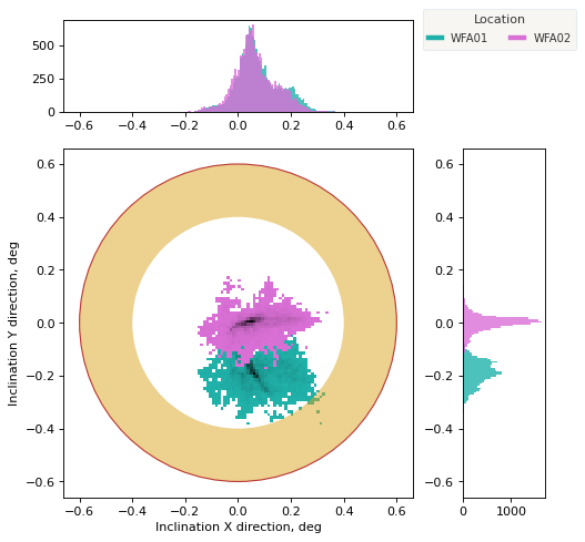
plt.rcParams.update({"axes.grid": False})
# Example plotting of the inclinations in the X and Y directions, with marginal
# histograms and alarm/warning levels.
def CustomCmap(from_rgb,to_rgb):
"""Create a custom colormap from two RGB tuples."""
r1, g1, b1 = from_rgb
r2, g2, b2 = to_rgb
cdict = {'red': ((0, r1, r1), (1, r2, r2)),
'green': ((0, g1, g1), (1, g2, g2)),
'blue': ((0, b1, b1), (1, b2, b2))}
cmap = mcolors.LinearSegmentedColormap('custom_cmap', cdict)
return cmap
# # ** Parameters **
MAIN_AXES_TITLE_FONT_SIZE = 10
TICK_LABEL_FONT_SIZE = 9
X_PARAMETER = "mean_TP_INC_LAT015_DEG240_X_nr1"
Y_PARAMETER = "mean_TP_INC_LAT015_DEG240_Y_nr2"
X_AXIS_TITLE = "Inclination X direction, deg"
Y_AXIS_TITLE = "Inclination Y direction, deg"
ALARM_LEVEL = 0.6
WARNING_LEVEL = 0.4
WARNING_WIDTH = ALARM_LEVEL - WARNING_LEVEL
LIM = ALARM_LEVEL * 1.1
# **Plotting**
fig2 = plt.figure(figsize=(7, 7), dpi=80)
# Define the grid layout
grid = plt.GridSpec(4, 4, hspace=0.4, wspace=0.6)
# Main plot (2D KDE)
main_ax = fig2.add_subplot(grid[1:4, 0:3])
# Marginal KDE plots
x_hist = fig2.add_subplot(grid[0, 0:3], sharex=main_ax);
y_hist = fig2.add_subplot(grid[1:4, 3], sharey=main_ax);
# Color settings
colors = ["lightseagreen", "orchid", "teal", "purple", "skyblue", "coral",
"gold", "darkkhaki", "lightcoral", "thistle", "lime", "darkorange",
"darkgreen", "deeppink", "navy"]
color_cycle = iter(colors)
legend_patches = []
for i, (location, group) in enumerate(data_ss.groupby("location")):
try:
color = next(color_cycle)
except StopIteration:
color_cycle = iter(colors)
color = next(color_cycle)
# 2D histogram on main_ax
rgb_color = mcolors.to_rgb(color)
light_rgb_color = tuple([c * 1 for c in rgb_color])
dark_rgb_color = tuple([c * 0.05 for c in rgb_color])
custom_cmap = CustomCmap(light_rgb_color, dark_rgb_color)
custom_cmap.set_under((1, 1, 1, 0))
h2d = main_ax.hist2d(group[X_PARAMETER], group[Y_PARAMETER], bins=120,
range=[[-LIM, LIM], [-LIM, LIM]], cmap=custom_cmap,
vmin=1, density=True)
# Marginal histogram for X axis
x_hist.hist(group[X_PARAMETER], bins=200, range=(-LIM, LIM), color=color,
alpha=0.8)
# Marginal histogram for Y axis (horizontal)
y_hist.hist(group[Y_PARAMETER], bins=200, range=(-LIM, LIM), color=color,
orientation='horizontal', alpha=0.8)
legend_patches.append(plt.Line2D([], [], color=color, lw=4, label=location))
# Draw alarm and warning levels
main_ax.add_patch(Wedge(center=(0, 0), r=ALARM_LEVEL, theta1=0, theta2=360,
width=WARNING_WIDTH, alpha=0.5, facecolor="goldenrod",
fill=True, linewidth=2, label='Warning Level'))
main_ax.add_patch(plt.Circle((0, 0), ALARM_LEVEL, edgecolor='firebrick',
alpha=0.9, fill=False, label="Alarm"))
x_hist.set_xlabel("");
y_hist.set_ylabel("");
# # Legend styling
legend = main_ax.legend(handles=legend_patches, loc="upper center",
title="Location", fontsize=TICK_LABEL_FONT_SIZE,
title_fontsize=10, frameon=True, facecolor="#F5F4EF",
edgecolor='#e4e8ee', bbox_to_anchor=(1.25, 1.4),
borderaxespad=0, labelspacing=0.7, handlelength=1.2,
borderpad=0.5, framealpha=0.8, fancybox=True,
shadow=False, ncol=6)
# Set legend font color
plt.setp(legend.get_texts(), color="#333333") # Labels in legend
plt.setp(legend.get_title(), color="#333333") # Title in legend
# Axis labels
main_ax.set_xlabel(X_AXIS_TITLE, fontsize=MAIN_AXES_TITLE_FONT_SIZE)
main_ax.set_ylabel(Y_AXIS_TITLE, fontsize=MAIN_AXES_TITLE_FONT_SIZE)
plt.show()
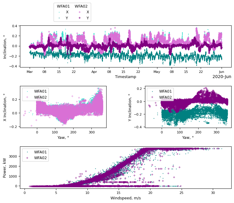
[9]:
# Example plotting of the inclinations in the X and Y directions V. timestamp,
# and yaw as well as the power curve.

fig = plt.figure(figsize=(9, 7))

gs = fig.add_gridspec(19, 12)
ax1 = fig.add_subplot(gs[0:5, :])
ax2 = fig.add_subplot(gs[7:12, 0:5])
ax3 = fig.add_subplot(gs[7:12, 7:])
ax4 = fig.add_subplot(gs[14:, :])
FONT_SIZE = 9

# Inclination V. Timestamp
ax_1 = df.plot("timestamp", "mean_WF_A01_TP_INC_LAT015_DEG240_X_nr1",
              kind="scatter", color="turquoise", marker=".", label="X", s=2,
              ax=ax1)
df.plot("timestamp", "mean_WF_A01_TP_INC_LAT015_DEG240_Y_nr2",
        kind="scatter", color="teal", marker=".", ax=ax_1, s=2,
        label="Y")
df.plot("timestamp", "mean_WF_A02_TP_INC_LAT015_DEG240_X_nr1",
        kind="scatter", color="orchid", marker="+", ax=ax_1, alpha=0.7,
        label="X")
df.plot("timestamp", "mean_WF_A02_TP_INC_LAT015_DEG240_Y_nr2",
        kind="scatter", color="purple", marker="+", ax=ax_1, alpha=0.7,
        label="Y")
ax_1.legend(title="WFA01    WFA02", ncol=2, bbox_to_anchor=(0.15, 1.05),
            fontsize=FONT_SIZE, title_fontsize=FONT_SIZE)

locator = mdates.AutoDateLocator(minticks=20, maxticks=26)
formatter = mdates.ConciseDateFormatter(locator)
ax1.xaxis.set_major_locator(locator)
ax1.xaxis.set_major_formatter(formatter)
ax1.set_xlabel("Timestamp", fontsize=FONT_SIZE)
ax1.set_ylabel("Inclination, °", fontsize=FONT_SIZE)
ax1.tick_params(labelsize=int(FONT_SIZE-1))

# Inclination V. Yaw
df.plot("mean_WF_A01_yaw", "mean_WF_A01_TP_INC_LAT015_DEG240_X_nr1",
        kind="scatter", color="turquoise", marker=".", ax=ax2, s=2,
        label= "WFA01")
df.plot("mean_WF_A02_yaw", "mean_WF_A02_TP_INC_LAT015_DEG240_X_nr1",
        kind="scatter", color="orchid", marker="+", ax=ax2, alpha=0.5,
        label="WFA02")
df.plot("mean_WF_A01_yaw", "mean_WF_A01_TP_INC_LAT015_DEG240_Y_nr2",
        kind="scatter", color="teal", marker=".", ax=ax3, s=2,
        label="WFA01")
df.plot("mean_WF_A02_yaw", "mean_WF_A02_TP_INC_LAT015_DEG240_Y_nr2",
        kind="scatter", color="purple", marker="+", ax=ax3, alpha=0.5,
        label="WFA02")
ax2.legend(loc="upper left", fontsize=FONT_SIZE)
ax2.set_xlabel("Yaw, °", fontsize=FONT_SIZE)
ax2.set_ylabel("X Inclination, °", fontsize=FONT_SIZE)
ax2.tick_params(labelsize=int(FONT_SIZE-1))
ax3.legend(loc="upper left", fontsize=FONT_SIZE)
ax3.set_xlabel("Yaw, °", fontsize=FONT_SIZE)
ax3.set_ylabel("Y Inclination, °", fontsize=FONT_SIZE)
ax3.tick_params(labelsize=int(FONT_SIZE-1))

# Power V. Windspeed
df.plot("mean_WF_A01_windspeed", "mean_WF_A01_power",
        kind="scatter", color="teal", marker=".", ax=ax4, s=2,
        label="WFA01")
df.plot("mean_WF_A02_windspeed", "mean_WF_A02_power",
        kind="scatter", color="purple", marker="+", ax=ax4, alpha=0.5,
        label="WFA02")
ax4.legend(loc="upper left", fontsize=FONT_SIZE)
ax4.set_xlabel("Windspeed, m/s", fontsize=FONT_SIZE)
ax4.set_ylabel("Power, kW", fontsize=FONT_SIZE)
ax4.tick_params(labelsize=int(FONT_SIZE-1))

plt.show()
Category-Value Format#
Data can also be converted to a category-value format, where each metric is converted to a “category” column containing the metric name, and a “value” column containing the metric value. The site and location columns are added as dimensions. The resulting DataFrame is indexed by timestamp and sorted by index.
[10]:
from api_24sea.datasignals.core import to_category_value
data_cv = to_category_value(df, df.datasignals.selected_metrics.reset_index())
data_cv
Both index and column named 'timestamp' found. Index takes precedence.
/home/pietro.dantuono@24SEA.local/Projects/API-24SEA/api-24sea-pkg/api_24sea/datasignals/core.py:1675: FutureWarning: Downcasting object dtype arrays on .fillna, .ffill, .bfill is deprecated and will change in a future version. Call result.infer_objects(copy=False) instead. To opt-in to the future behavior, set `pd.set_option('future.no_silent_downcasting', True)`
  .bfill(axis=1)
[10]:
| timestamp | metric | value | unit | statistic | short_hand | site_id | location_id | sub_assembly | lat | heading | site | location | metric_group | |
|---|---|---|---|---|---|---|---|---|---|---|---|---|---|---|
| 0 | 2020-03-01 00:00:00+00:00 | mean_WF_A01_pitch | 66.398788 | ° | mean | pitch | WF | A01 | NaN | NaN | NaN | WindFarm | WFA01 | scada |
| 1 | 2020-03-01 00:10:00+00:00 | mean_WF_A01_pitch | 66.398788 | ° | mean | pitch | WF | A01 | NaN | NaN | NaN | WindFarm | WFA01 | scada |
| 2 | 2020-03-01 00:20:00+00:00 | mean_WF_A01_pitch | 66.398788 | ° | mean | pitch | WF | A01 | NaN | NaN | NaN | WindFarm | WFA01 | scada |
| 3 | 2020-03-01 00:30:00+00:00 | mean_WF_A01_pitch | 66.398788 | ° | mean | pitch | WF | A01 | NaN | NaN | NaN | WindFarm | WFA01 | scada |
| 4 | 2020-03-01 00:40:00+00:00 | mean_WF_A01_pitch | 66.398788 | ° | mean | pitch | WF | A01 | NaN | NaN | NaN | WindFarm | WFA01 | scada |
| ... | ... | ... | ... | ... | ... | ... | ... | ... | ... | ... | ... | ... | ... | ... |
| 211963 | 2020-05-31 23:10:00+00:00 | mean_WF_A02_TP_INC_LAT015_DEG240_Y_nr2 | -0.023932 | ° | mean | TP_INC_LAT015_DEG240_Y_nr2 | WF | A02 | TP | 15.0 | 240.0 | WindFarm | WFA02 | inclination |
| 211964 | 2020-05-31 23:20:00+00:00 | mean_WF_A02_TP_INC_LAT015_DEG240_Y_nr2 | -0.027713 | ° | mean | TP_INC_LAT015_DEG240_Y_nr2 | WF | A02 | TP | 15.0 | 240.0 | WindFarm | WFA02 | inclination |
| 211965 | 2020-05-31 23:30:00+00:00 | mean_WF_A02_TP_INC_LAT015_DEG240_Y_nr2 | -0.029176 | ° | mean | TP_INC_LAT015_DEG240_Y_nr2 | WF | A02 | TP | 15.0 | 240.0 | WindFarm | WFA02 | inclination |
| 211966 | 2020-05-31 23:40:00+00:00 | mean_WF_A02_TP_INC_LAT015_DEG240_Y_nr2 | -0.024185 | ° | mean | TP_INC_LAT015_DEG240_Y_nr2 | WF | A02 | TP | 15.0 | 240.0 | WindFarm | WFA02 | inclination |
| 211967 | 2020-05-31 23:50:00+00:00 | mean_WF_A02_TP_INC_LAT015_DEG240_Y_nr2 | -0.030792 | ° | mean | TP_INC_LAT015_DEG240_Y_nr2 | WF | A02 | TP | 15.0 | 240.0 | WindFarm | WFA02 | inclination |
211968 rows × 14 columns